Plotting gASCA results with ggplot and tidyverse

Introduction

In the ASCA Decomposition of Synthetic Count Data vignette we showed how to run and visualize an ASCA decomposition relying on base graphics. However, visualizations are often performed using tidyverse and ggplot.

The aim of this article is to show how to visualize the results of an ASCA decomposition using these packages. As in the previous case we will use the synthetic data made available in the package:

## load the libraries
library(gASCA)
library(tidyverse)
library(patchwork)   ## to combine the ggplots in complex figures

library(ggrepel)


## load the dataset
data("synth_count_data")

The following plot shows the distribution of the counts for variables s1 and s7 as a function of the design factors:

tibble(synth_count_data$design,
       data.frame(synth_count_data$counts)) %>% 
  pivot_longer(starts_with("s")) %>% 
  filter(name %in% c("s1","s7")) %>% 
  ggplot() + 
  geom_point(aes(x = time, y = value, col = treatment),
             position = position_jitterdodge(dodge.width = 0.4, jitter.width = 0.05), pch = 19, size =2, alpha = 0.5) + 
  scale_color_brewer(palette = "Set1", name = "Treatment") + 
  scale_y_log10() + 
  facet_wrap(~name, scales = "free") +
  xlab("Time") + 
  theme_bw() + 
  theme(aspect.ratio = 0.5)

## Warning: Transformation introduced infinite values in continuous y-axis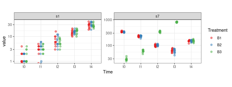

The effect of time on variable s1 is clear. The presence of an interaction between time and treatment is instead visible in the s7 profile.

Visualize the results of the decomposition and of the validation

Run the decomposition

## perform the decomposition
asca0 <- ASCA_decompose(
  d = synth_count_data$design,
  x = synth_count_data$counts, 
  f = "time + treatment + time:treatment",
  glm_par = list(family = poisson()))

Run the validation

The following plot shows the results of the decomposition and the validation in terms of L2 norm of the terms, the variable importance and the univariate pseudo-R2

figure2_term_val <- asca0_validation$L2_qt %>% 
  as_tibble(rownames = "term") %>% 
  add_column(actual = asca0$terms_L2) %>% 
  mutate(term = factor(term, levels = term)) %>% 
  ggplot() + 
  geom_col(aes(x = term, y = actual), fill = "steelblue") +
  geom_col(aes(x = term, y = value), fill = "darkred") +
  ylab("term-L2") + xlab("") + 
  theme_bw() +
  theme(axis.text.x = element_text(size=8),
        axis.text.y = element_text(size=8))
  

figure2_varimp_val <- asca0$varimp %>% 
  as_tibble(rownames = "var") %>% 
  pivot_longer(-var) %>% 
  left_join(asca0_validation$varimp_qt %>% 
              as_tibble(rownames = "var") %>% 
              pivot_longer(-var, values_to = "value_qt")) %>% 
  mutate(var = factor(var, levels = unique(var))) %>% 
  mutate(name = factor(name, levels = unique(name))) %>% 
  ggplot() + 
  geom_col(aes(x = var, y = value), fill = "steelblue") +
  geom_col(aes(x = var, y = value_qt), fill = "darkred") +
  facet_wrap(~name, scales = "free", nrow = 1) +
  ylab("Vecror Norm") + xlab("") + 
  theme_bw() +
  theme(axis.text.x = element_text(size=8, angle = 45, vjust = 1, hjust=1),
        axis.text.y = element_text(size=8))

## Joining, by = c("var", "name")

figure2_R2_val <- asca0_validation$R2_qt %>% 
  as_tibble(rownames = "var") %>%  
  add_column(actual = asca0$pseudoR2) %>% 
  mutate(var = factor(var, levels = unique(var))) %>% 
  ggplot() + 
  geom_col(aes(x = var, y = actual), fill = "steelblue") +
  geom_col(aes(x = var, y = value), fill = "darkred") +
  ylab("pseudo-R2") + xlab("") + 
  theme_bw() +
  theme(axis.text.x = element_text(size=8),
        axis.text.y = element_text(size=8))

## Define the layout
layout <- "
ABB
CCC
"

## prepare the figure
figure2_term_val + 
  figure2_R2_val + 
  figure2_varimp_val +   
  plot_annotation(tag_levels = 'a') + 
  plot_layout(heights = unit(c(3,4.5),"cm"), widths =  unit(c(6,7),"cm"), design = layout)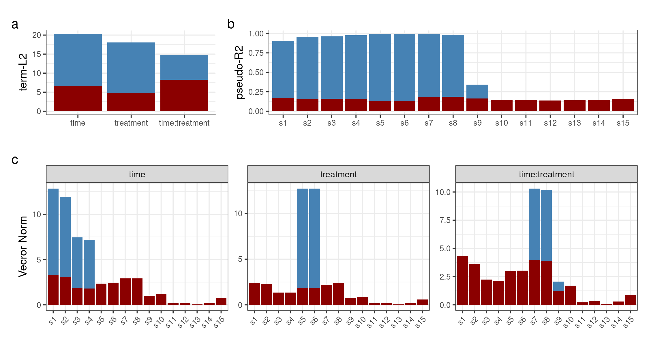

Visualization of the decomposition terms

Perform the decomposition

asca0_svd <- ASCA_svd(ASCA_trim_vars(asca0$decomposition, keep = 1:10))

Visualize screeplots, LVs and loadings

Screeplot

## here we make a scree plot of the three decomposition terms
screeplot <- map(asca0_svd, ~ .x$sdev %>% as_tibble(., rownames = "PC")) %>% 
  enframe(name = "term", value = "data") %>%
  # mutate(data = map(data,~ .x %>% mutate(value = (value/sum(value))*100))) %>% 
  unnest(cols = c(data)) %>% 
  mutate(PC = factor(PC, levels = unique(PC))) %>% 
  mutate(term = factor(term, levels = c("time","treatment","time:treatment"))) %>% 
  filter(PC %in% as.character(1:6)) %>% 
  ggplot() + 
  geom_col(aes(x = PC, y = value^2), fill = "steelblue") + 
  facet_wrap(~term, scales = "free", ncol = 3) + 
  ylab("Variances") + 
  xlab("LV") + 
  theme_bw() + 
  theme(aspect.ratio = 0.4)

LVs

LV_plot <- cbind.data.frame(time_LV1 = asca0_svd$time$x[,1],
                 time_LV2 = asca0_svd$time$x[,2],
                 treatment_LV1 = asca0_svd$treatment$x[,1],
                 "time:treat_LV1" = asca0_svd$`time:treatment`$x[,1], 
                 "time:treat_LV2" = asca0_svd$`time:treatment`$x[,2]) %>% 
  mutate(across(everything(),~round(.x,2))) %>%     
  add_column(synth_count_data$design) %>% 
  pivot_longer(contains("LV")) %>% 
  unique() %>% 
  mutate(name = factor(name)) %>% 
  mutate(name = fct_relevel(name, "treatment_LV1", after = 2)) %>% 
  ggplot() +
  geom_point(aes(x = time, y = value, col = treatment), alpha = 0.5, size = 3) + 
  geom_line(aes(x = time, y = value, col = treatment, group = treatment, lty = treatment)) + 
  facet_wrap(~name, ncol = 1, scales = "free_y") + 
  scale_color_brewer(palette = "Set1") +
  theme_bw() + 
  theme(aspect.ratio = 0.3, legend.position = "bottom")

Loadings

loading_plot <- cbind.data.frame(time_LV1 = asca0_svd$time$rotation[,1],
                 time_LV2 = asca0_svd$time$rotation[,2],
                 treatment_LV1 = asca0_svd$treatment$rotation[,1],
                 "time:treat_LV1" = asca0_svd$`time:treatment`$rotation[,1], 
                 "time:treat_LV2" = asca0_svd$`time:treatment`$rotation[,2]) %>% 
  add_column(species = paste0("s",1:10)) %>% 
  mutate(species = factor(species, levels = paste0("s",1:10))) %>% 
  pivot_longer(contains("LV")) %>% 
  mutate(name = factor(name)) %>% 
  mutate(name = fct_relevel(name, "treatment_LV1", after = 2)) %>% 
  ggplot() +
  geom_col(aes(x = species, y = value), fill = "steelblue") + 
  geom_hline(yintercept = 0, lty = 2) + 
  facet_wrap(~name, ncol = 1) + 
  theme_bw() + 
  theme(aspect.ratio = 0.4)

Combined Figure

## Define the layout
layout <- "
AAAA
BBCC
"

## prepare the figure
screeplot + 
  LV_plot + 
  loading_plot +   
  plot_annotation(tag_levels = 'a') + 
  plot_layout(heights = unit(c(3,13),"cm"), widths =  unit(c(4,3),"cm"), design = layout)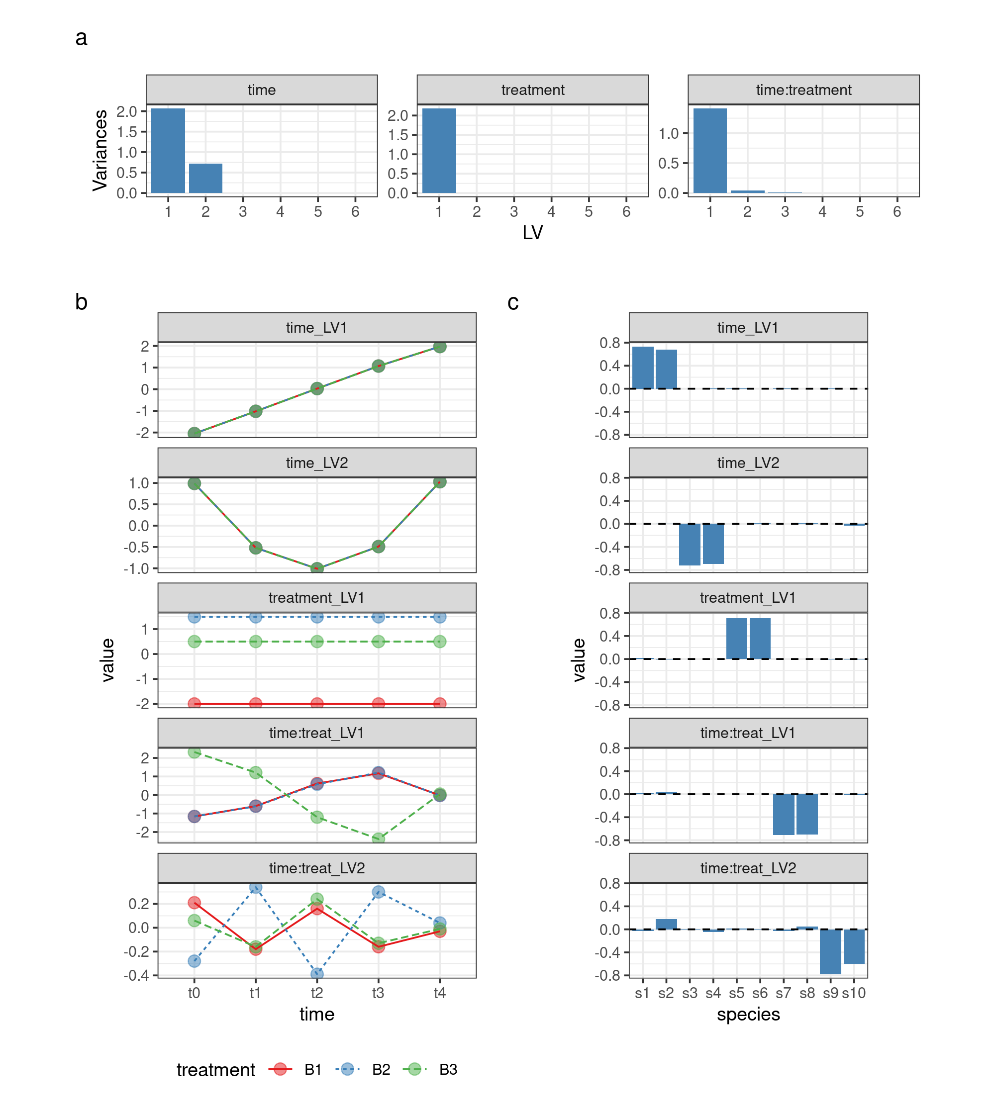

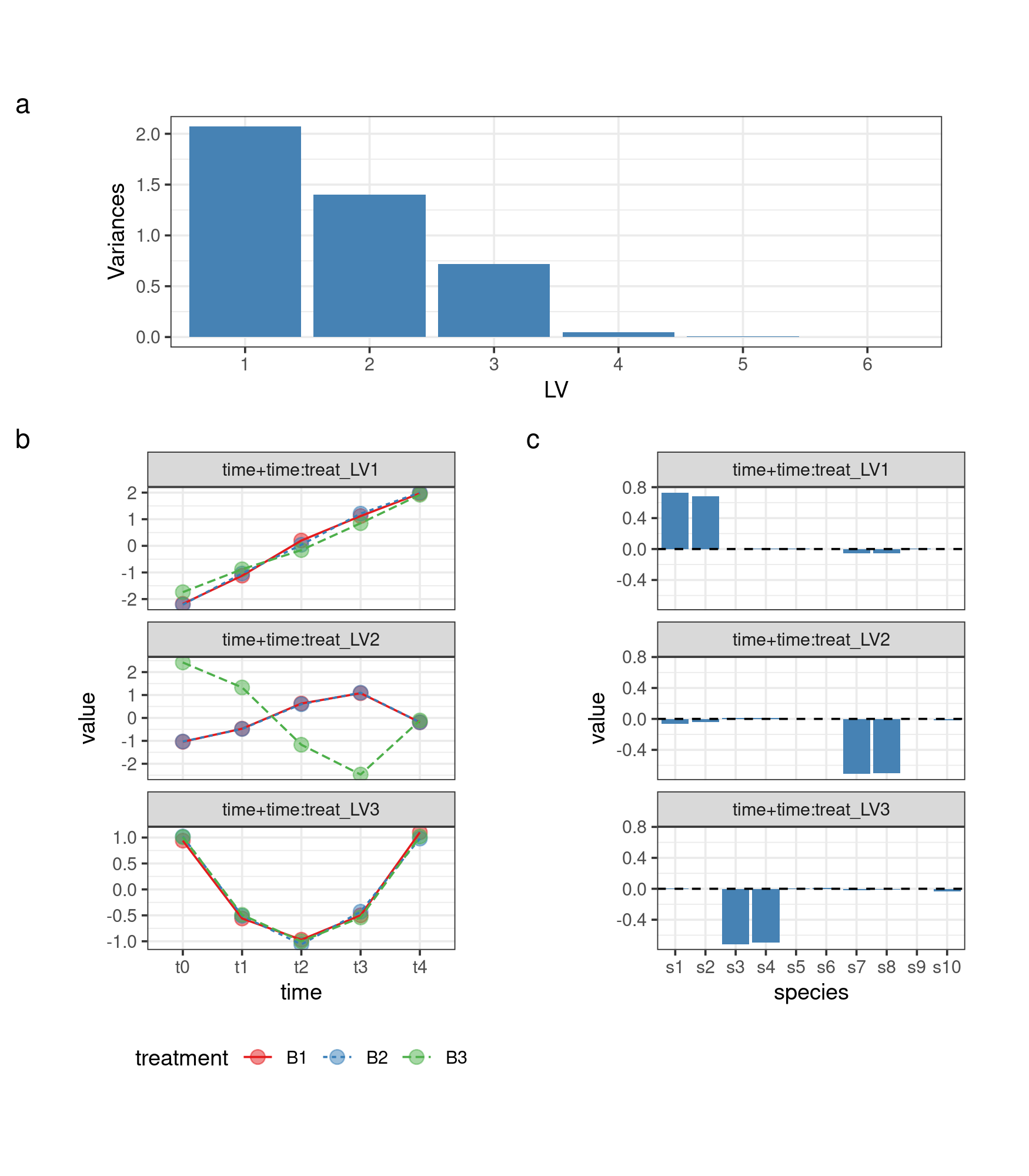
Combining terms

The function ASCA_combine_terms allows the combination of different factor matrices. The function accepts as input the output of ASCA_decomposition and a character vector specifying which terms should be combined.

## combine two terms
asca0_comb <- ASCA_combine_terms(asca0, c("time","time:treatment"))

## perform the svd of the combined decomposition 
asca0_comb_svd <- ASCA_svd(ASCA_trim_vars(asca0_comb$decomposition, keep = 1:10))

Visualize screeplot LVs and Loadings of the combined term

Screeplot

## here we make a scree plot of the three decomposition terms
screeplot_comb <- asca0_comb_svd$`time+time:treatment`$sdev %>% 
  as_tibble(., rownames = "PC") %>% 
  mutate(PC = factor(PC, levels = unique(PC))) %>% 
  filter(PC %in% as.character(1:6)) %>% 
  ggplot() + 
  geom_col(aes(x = PC, y = value^2), fill = "steelblue") + 
  ylab("Variances") + 
  xlab("LV") + 
  theme_bw() + 
  theme(aspect.ratio = 0.3)

LVs

LV_plot_comb <- cbind.data.frame("time+time:treat_LV1" = asca0_comb_svd$`time+time:treatment`$x[,1], 
                                 "time+time:treat_LV2" = asca0_comb_svd$`time+time:treatment`$x[,2],
                                 "time+time:treat_LV3" = asca0_comb_svd$`time+time:treatment`$x[,3]) %>% 
  mutate(across(everything(),~round(.x,2))) %>%     
  add_column(synth_count_data$design) %>% 
  pivot_longer(contains("LV")) %>% 
  unique() %>% 
  mutate(name = factor(name)) %>% 
  ggplot() +
  geom_point(aes(x = time, y = value, col = treatment), alpha = 0.5, size = 3) + 
  geom_line(aes(x = time, y = value, col = treatment, group = treatment, lty = treatment)) + 
  facet_wrap(~name, ncol = 1, scales = "free_y") + 
  scale_color_brewer(palette = "Set1") +
  theme_bw() + 
  theme(aspect.ratio = 0.4, legend.position = "bottom")

Loadings

loading_plot_comb <- cbind.data.frame("time+time:treat_LV1" = asca0_comb_svd$`time+time:treatment`$rotation[,1], 
                                 "time+time:treat_LV2" = asca0_comb_svd$`time+time:treatment`$rotation[,2],
                                 "time+time:treat_LV3" = asca0_comb_svd$`time+time:treatment`$rotation[,3]) %>% 
  add_column(species = paste0("s",1:10)) %>% 
  mutate(species = factor(species, levels = paste0("s",1:10))) %>% 
  pivot_longer(contains("LV")) %>% 
  mutate(name = factor(name)) %>% 
  ggplot() +
  geom_col(aes(x = species, y = value), fill = "steelblue") + 
  geom_hline(yintercept = 0, lty = 2) + 
  facet_wrap(~name, ncol = 1) + 
  theme_bw() + 
  theme(aspect.ratio = 0.4)

combined Figure

## Define the layout
layout <- "
AAAA
BBCC
"

## prepare the figure
screeplot_comb + 
  LV_plot_comb + 
  loading_plot_comb +   
  plot_annotation(tag_levels = 'a') + 
  plot_layout(heights = unit(c(4,8),"cm"), widths =  unit(c(3.5,3.5),"cm"), design = layout)

Pietro Franceschi

Introduction

Visualize the results of the decomposition and of the validation

Run the decomposition

Run the validation

Visualization of the decomposition terms

Perform the decomposition

Visualize screeplots, LVs and loadings

Screeplot

LVs

Loadings

Combined Figure

Combining terms

Visualize screeplot LVs and Loadings of the combined term

Screeplot

LVs

Loadings

combined Figure